Light curves

AMPy can generate multi-band light curves from observational data and model predictions. The light curve routine is model-agnostic and works with any built-in or user-defined model, including arbitrary plugin combinations.

Observed data are plotted alongside the inferred model, with bands color-coded using the Band column from the input file.

Basic usage

The easiest way to generate a light curve is through the high-level AMPy interface:

ampy.lightcurve()

If inference has already been run, this uses the best-fit parameters from the most recent inference result stored on the ampy instance and overlays the corresponding model prediction on the data.

Uncertainty regions

AMPy can display an uncertainty region using posterior samples from the inference. To plot a shaded region corresponding to a given confidence level:

ampy.lightcurve(sigma=1)

Here, sigma=1 corresponds to a 1σ uncertainty region.

Calibration offsets

By default, calibration offsets (if modeled) are not applied when plotting. This allows users to visualize the raw observational data. To apply calibration offsets to the plotted data:

ampy.lightcurve(offset=True)

This is useful when assessing the calibrated agreement between model and data.

Advanced Usage

For more control—such as generating a model light curve from user-specified parameters without running inference—use the lower-level generator function:

from ampy.products.plotting import generate_light_curve

ax = generate_light_curve(obs=obs, plugins=plugins, params=params)

This function can be called directly in scripts to generate dense model curves (e.g., ndata points per band), apply optional band spreading, or customize Matplotlib plotting options via ll_kwargs and plot_kwargs.

See the plotting API reference for full details.

Example output

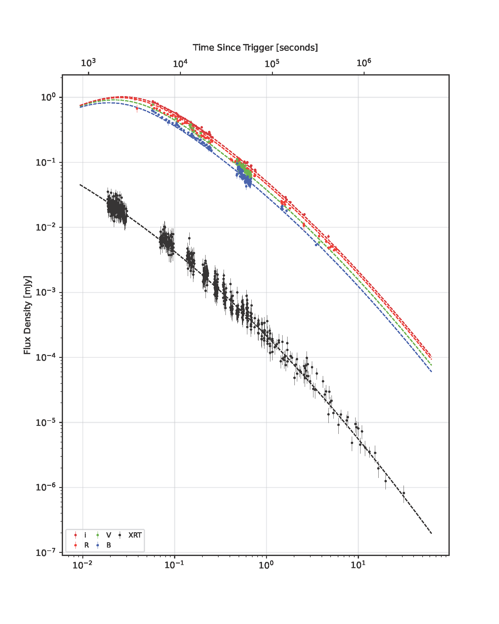
../../_images/ex_lightcurve.png — Example multi-band light curve generated by AMPy using default settings. `Download PDF`